Steps 1-6
- Load the R packages we will use.
- Read the data in the files ‘drugs_cos.tsv’ , ‘health.csv’ in to R and assign to the variables ‘drug_cos’ and ‘health_cos’ , respectively.
drug_cos  <- read_csv("https://estanny.com/static/week6/drug_cos.csv")

health_cos  <- read_csv("https://estanny.com/static/week6/health_cos.csv")
- use ‘glimpse’ to get a glimpse of the data.
drug_cos %>% glimpse()
Rows: 104
Columns: 9
$ ticker       <chr> "ZTS", "ZTS", "ZTS", "ZTS", "ZTS", "ZTS", "Z...
$ name         <chr> "Zoetis Inc", "Zoetis Inc", "Zoetis Inc", "Z...
$ location     <chr> "New Jersey; U.S.A", "New Jersey; U.S.A", "N...
$ ebitdamargin <dbl> 0.149, 0.217, 0.222, 0.238, 0.182, 0.335, 0....
$ grossmargin  <dbl> 0.610, 0.640, 0.634, 0.641, 0.635, 0.659, 0....
$ netmargin    <dbl> 0.058, 0.101, 0.111, 0.122, 0.071, 0.168, 0....
$ ros          <dbl> 0.101, 0.171, 0.176, 0.195, 0.140, 0.286, 0....
$ roe          <dbl> 0.069, 0.113, 0.612, 0.465, 0.285, 0.587, 0....
$ year         <dbl> 2011, 2012, 2013, 2014, 2015, 2016, 2017, 20...
health_cos %>% glimpse()
Rows: 464
Columns: 11
$ ticker      <chr> "ZTS", "ZTS", "ZTS", "ZTS", "ZTS", "ZTS", "ZT...
$ name        <chr> "Zoetis Inc", "Zoetis Inc", "Zoetis Inc", "Zo...
$ revenue     <dbl> 4233000000, 4336000000, 4561000000, 478500000...
$ gp          <dbl> 2581000000, 2773000000, 2892000000, 306800000...
$ rnd         <dbl> 427000000, 409000000, 399000000, 396000000, 3...
$ netincome   <dbl> 245000000, 436000000, 504000000, 583000000, 3...
$ assets      <dbl> 5711000000, 6262000000, 6558000000, 658800000...
$ liabilities <dbl> 1975000000, 2221000000, 5596000000, 525100000...
$ marketcap   <dbl> NA, NA, 16345223371, 21572007994, 23860348635...
$ year        <dbl> 2011, 2012, 2013, 2014, 2015, 2016, 2017, 201...
$ industry <chr> "Drug Manufacturers - Specialty & Generic", "...- Which variables are the same in both data sets.
names_drug  <- drug_cos  %>%  names()
names_health  <- health_cos %>% names()
intersect(names_drug, names_health)
[1] "ticker" "name" "year" - Select subset of variables to work with.
For ‘drug_cos’ select ‘ticker’, ‘year’, ‘grossmargin’
Extract observations for 2018
Assign output to ‘drug_subset’
For ‘health_cos’ select ‘ticker’, ‘year’, ‘revenue’, ‘gp’, ‘industry’
Extract observation for 2018
Assign output to ‘health_subset’
drug_subset  <- drug_cos  %>%
  select(ticker, year, grossmargin)  %>%
  filter(year == 2018)
health_subset  <- health_cos  %>%
  select(ticker, year, revenue, gp, industry)  %>%
  filter(year == 2018)
- Keep all the rows and columns ‘drug_select’ join with columns in ‘health_subset’
drug_subset %>% left_join(health_subset)
# A tibble: 13 x 6
   ticker  year grossmargin   revenue        gp industry
   <chr>  <dbl>       <dbl>     <dbl>     <dbl> <chr>
 1 ZTS     2018       0.672   5.82e 9   3.91e 9 Drug Manufacturers - ~
 2 PRGO    2018       0.387   4.73e 9   1.83e 9 Drug Manufacturers - ~
 3 PFE     2018       0.79    5.36e10   4.24e10 Drug Manufacturers - ~
 4 MYL     2018       0.35    1.14e10   4.00e 9 Drug Manufacturers - ~
 5 MRK     2018       0.681   4.23e10   2.88e10 Drug Manufacturers - ~
 6 LLY     2018       0.738   2.46e10   1.81e10 Drug Manufacturers - ~
 7 JNJ     2018       0.668   8.16e10   5.45e10 Drug Manufacturers - ~
 8 GILD    2018       0.781   2.21e10   1.73e10 Drug Manufacturers - ~
 9 BMY     2018       0.71    2.26e10   1.60e10 Drug Manufacturers - ~
10 BIIB    2018       0.865   1.35e10   1.16e10 Drug Manufacturers - ~
11 AMGN    2018       0.827   2.37e10   1.96e10 Drug Manufacturers - ~
12 AGN     2018       0.861   1.58e10   1.36e10 Drug Manufacturers - ~
13 ABBV    2018       0.764   3.28e10   2.50e10 Drug Manufacturers - ~
Question join_ticker
Start with ‘drug_cos’
Extract observations for the ticker JNJ from ‘durg_cos’
Assign output to the variable ‘drug_cos_subset’
drug_cos_subset  <- drug_cos  %>%
  filter(ticker == "JNJ")
- Display’ ‘drug_cos_subset’
drug_cos_subset
# A tibble: 8 x 9
  ticker name  location ebitdamargin grossmargin netmargin   ros   roe
  <chr>  <chr> <chr>           <dbl>       <dbl>     <dbl> <dbl> <dbl>
1 JNJ    John~ New Jer~        0.247       0.687     0.149 0.199 0.161
2 JNJ    John~ New Jer~        0.272       0.678     0.161 0.218 0.173
3 JNJ    John~ New Jer~        0.281       0.687     0.194 0.224 0.197
4 JNJ    John~ New Jer~        0.336       0.694     0.22  0.284 0.217
5 JNJ    John~ New Jer~        0.335       0.693     0.22  0.282 0.219
6 JNJ    John~ New Jer~        0.338       0.697     0.23  0.286 0.229
7 JNJ    John~ New Jer~        0.317       0.667     0.017 0.243 0.019
8 JNJ    John~ New Jer~        0.318       0.668     0.188 0.233 0.244
# ... with 1 more variable: year <dbl>
Use left_join to combine the rows and columns of ‘drug_cos_subset’ with the columns of ‘health_cos’
Assign the output to ‘combo_df’
combo_df  <-  drug_cos_subset  %>%
  left_join(health_cos)
- Display ‘combo_df’
combo_df# A tibble: 8 x 17 ticker name location ebitdamargin grossmargin netmargin ros roe <chr> <chr> <chr> <dbl> <dbl> <dbl> <dbl> <dbl> 1 JNJ John~ New Jer~ 0.247 0.687 0.149 0.199 0.161 2 JNJ John~ New Jer~ 0.272 0.678 0.161 0.218 0.173 3 JNJ John~ New Jer~ 0.281 0.687 0.194 0.224 0.197 4 JNJ John~ New Jer~ 0.336 0.694 0.22 0.284 0.217 5 JNJ John~ New Jer~ 0.335 0.693 0.22 0.282 0.219 6 JNJ John~ New Jer~ 0.338 0.697 0.23 0.286 0.229 7 JNJ John~ New Jer~ 0.317 0.667 0.017 0.243 0.019 8 JNJ John~ New Jer~ 0.318 0.668 0.188 0.233 0.244 # ... with 9 more variables: year <dbl>, revenue <dbl>, gp <dbl>, # rnd <dbl>, netincome <dbl>, assets <dbl>, liabilities <dbl>, # marketcap <dbl>, industry <chr>- note: the variables ‘ticker’, ‘name’, ‘location’ and ‘industry’ are the same for all the observations.
- Assign the company name to ‘co_name’
co_name  <-  combo_df  %>%
  distinct(name)  %>%
  pull()
- Assign the company location to’ co_location’
co_location <- combo_df %>% distinct(location) %>% pull()- Assign the company location to’ co_industry’
co_industry  <-  combo_df  %>%
  distinct(industry)  %>%
  pull()
Put the r inline commands used in the blanks below. When you knit the document the results of the commands will be displayed in your text.
The company JNJ is located in New Jersey and is a member of the drug manufacturers- general group.
Start with ‘combo_df’
Select variables ‘year’, ‘grossmargin’, ‘netmargin’, ‘revenue’, ‘gp’, ‘netmargin’
combo_of_subset  <- combo_df  %>%
  select(year, grossmargin, netmargin, revenue, gp, netmargin)
- Display ‘combo_of_subset’
combo_of_subset# A tibble: 8 x 5 year grossmargin netmargin revenue gp <dbl> <dbl> <dbl> <dbl> <dbl> 1 2011 0.687 0.149 65030000000 44670000000 2 2012 0.678 0.161 67224000000 45566000000 3 2013 0.687 0.194 71312000000 48970000000 4 2014 0.694 0.22 74331000000 51585000000 5 2015 0.693 0.22 70074000000 48538000000 6 2016 0.697 0.23 71890000000 50101000000 7 2017 0.667 0.017 76450000000 51011000000 8 2018 0.668 0.188 81581000000 54490000000
Create the variable ‘grossmargin_check’ to compare with the variable ‘grossmargin’. They should be equal. ‘grossmargin_check’ = ‘gp’ / ‘revenue’ Create the variable ‘close_enough’ to check that the absolute value of the difference between ‘grossmargin_check’ and ‘grossmargin’ is less than 0.001
combo_of_subset  %>%
  mutate(grossmargin_check = gp/ revenue,
         close_enough = abs(grossmargin_check - grossmargin) < 0.001)
# A tibble: 8 x 7 year grossmargin netmargin revenue gp grossmargin_che~ <dbl> <dbl> <dbl> <dbl> <dbl> <dbl> 1 2011 0.687 0.149 6.50e10 4.47e10 0.687 2 2012 0.678 0.161 6.72e10 4.56e10 0.678 3 2013 0.687 0.194 7.13e10 4.90e10 0.687 4 2014 0.694 0.22 7.43e10 5.16e10 0.694 5 2015 0.693 0.22 7.01e10 4.85e10 0.693 6 2016 0.697 0.23 7.19e10 5.01e10 0.697 7 2017 0.667 0.017 7.64e10 5.10e10 0.667 8 2018 0.668 0.188 8.16e10 5.45e10 0.668 # ... with 1 more variable: close_enough <lgl>
Create the variable ‘netmargin_check’ to compare with the variable ‘netmargin’. They should be equal.
Create the variable ‘close_enough’ to check that the absolute value of the difference between ‘netmargin_check’ and ‘netmargin’ is less than 0.001
combo_of_subset  %>%
  mutate(netmargin_check = gp/ revenue,
         close_enough = abs(netmargin_check - netmargin) < 0.001)
# A tibble: 8 x 7 year grossmargin netmargin revenue gp netmargin_check <dbl> <dbl> <dbl> <dbl> <dbl> <dbl> 1 2011 0.687 0.149 6.50e10 4.47e10 0.687 2 2012 0.678 0.161 6.72e10 4.56e10 0.678 3 2013 0.687 0.194 7.13e10 4.90e10 0.687 4 2014 0.694 0.22 7.43e10 5.16e10 0.694 5 2015 0.693 0.22 7.01e10 4.85e10 0.693 6 2016 0.697 0.23 7.19e10 5.01e10 0.697 7 2017 0.667 0.017 7.64e10 5.10e10 0.667 8 2018 0.668 0.188 8.16e10 5.45e10 0.668 # ... with 1 more variable: close_enough <lgl>
Question: summarize_industry
Fill in the blanks
Put the command you use in the Rchunks in the Rmd file for this quiz
Use the health_cos data
For each industry calculate
mean_netmargin_percent = mean(netincome / revenue) * 100 median_netmargin_percent = median(netincome / revenue) * 100 min_netmargin_percent = min(netincome / revenue) * 100 max_netmargin_percent = max(netincome / revenue) * 100
health_cos %>%
  group_by(industry)  %>%
  summarize(mean_netmargin_percent = mean(netincome / revenue) * 100,
            median_netmargin_percent = median(netincome / revenue) * 100,
            min_netmargin_percent = min(netincome / revenue) * 100,
            max_netmargin_percent = max(netincome / revenue) * 100)
# A tibble: 9 x 5 industry mean_netmargin_~ median_netmargi~ min_netmargin_p~ * <chr> <dbl> <dbl> <dbl> 1 Biotech~ -4.66 7.62 -197. 2 Diagnos~ 13.1 12.3 0.399 3 Drug Ma~ 19.4 19.5 -34.9 4 Drug Ma~ 5.88 9.01 -76.0 5 Healthc~ 3.28 3.37 -0.305 6 Medical~ 6.10 6.46 1.40 7 Medical~ 12.4 14.3 -56.1 8 Medical~ 1.70 1.03 -0.102 9 Medical~ 12.3 14.0 -47.1 # ... with 1 more variable: max_netmargin_percent <dbl>mean_netmargin_percent for the industry Diagnostics & Research is 13.1%
median_netmargin_percent for the industry Diagnostics & Research is 12.3%
min_netmargin_percent for the industry Diagnostics & Research is .399%
max_netmargin_percent for the industry Diagnostics & Research is 26.3%
Question: inline_ticker
Fill in the blanks
Use the health_cos data
Extract observations for the ticker BMY from health_cos and assign to the variable health_cos_subset
health_cos_subset  <- health_cos  %>%
  filter(ticker == "BMY")
*Display ‘health_cos_subset_’
health_cos_subset# A tibble: 8 x 11 ticker name revenue gp rnd netincome assets liabilities <chr> <chr> <dbl> <dbl> <dbl> <dbl> <dbl> <dbl> 1 BMY Bris~ 2.12e10 1.56e10 3.84e9 3.71e9 3.30e10 17103000000 2 BMY Bris~ 1.76e10 1.30e10 3.90e9 1.96e9 3.59e10 22259000000 3 BMY Bris~ 1.64e10 1.18e10 3.73e9 2.56e9 3.86e10 23356000000 4 BMY Bris~ 1.59e10 1.19e10 4.53e9 2.00e9 3.37e10 18766000000 5 BMY Bris~ 1.66e10 1.27e10 5.92e9 1.56e9 3.17e10 17324000000 6 BMY Bris~ 1.94e10 1.45e10 5.01e9 4.46e9 3.37e10 17360000000 7 BMY Bris~ 2.08e10 1.47e10 6.48e9 1.01e9 3.36e10 21704000000 8 BMY Bris~ 2.26e10 1.60e10 6.34e9 4.92e9 3.50e10 20859000000 # ... with 3 more variables: marketcap <dbl>, year <dbl>, # industry <chr>In the console, type ‘?distinct’. Go to the help pane to see what distinct does
In the console, type ‘?pull’. Go to the help pane to see what pull does
Run the code below
health_cos_subset  %>%
  distinct(name) %>%
  pull(name)
[1] "Bristol Myers Squibb Co"- Assign the output to co_name
co_name  <-  health_cos_subset  %>%
  distinct(name) %>%
  pull(name)
You can take output from your code and include it in your text.
The name of the company with ticker BMY is Bristol Myers Squibb Co In following chuck
Assign the company’s industry group to the variable co_industry
co_industry  <-  health_cos_subset  %>%
  distinct(industry)  %>%
  pull()
The company Bristol Myers Squibb Co is a member of the drug manufacturers- general group. group.
- Prepare the data for the plots
- Start with ‘health_cos’ THEN
- group by industry. THEN
- calculate the median research and development expenditure by industry
- assign the group to ‘df’
- Use ‘glimpse’ to look at the data for the plot
df %>% glimpse()Rows: 9 Columns: 2 $ industry <chr> "Biotechnology", "Diagnostics & Research", "D... $ med_rnd_rev <dbl> 0.48317287, 0.05620271, 0.17451442, 0.0685187...- Create a static bar chart.
- use ‘ggplot’ to intialize the chart.
- data is ‘df’
- the ;variable ’industry id mapped to the x-axis
- reorder it based on ‘med_rnd_rev’
- ‘med_rnd_rev’ is set to the y-axis
- use ‘geomcol’ to add a bar chart
- use ’ scale_y-continuous to label the y_axis with percent
- use’ cord_flip to flip the coordinates
- use ‘labs’ to add title, subtitle and remove x and y axis
- use ‘themeipsum()’ from the hrbthemes package to improve the theme
ggplot(data = df, mapping = aes(
  x = reorder(industry, med_rnd_rev),
  y = med_rnd_rev
  )) +
  geom_col() +
  scale_y_continuous(labels = scales:: percent) +
  coord_flip() +
  labs(
    title = "Median R&D expenditures",
    subtitle = "by industrty as a percent of revenue from 2011 to 2018",
    x = NULL, y = NULL) +
  theme_ipsum()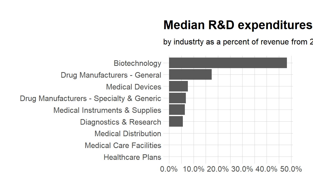
- Save the plot and add it to chunk at the top.
ggsave(filename = "preview.png",
       path = here::here("_posts", "2021-03-16-joining-data"))